Portfolio
Bioinformatics Lab Course @ UCSD
class13
Pooja Parthasarathy | A17817456
Background
Today we will perform an RNASeq analysis on the effects of dexamethasone (dex for short), a common steroid on airway smooth muscle (ASM) cell lines
Data
We need 2 things for this analysis - count and col data - countData: the biggest of the two, the table with genes as rows and samples as columns - **colData*: the metadata about the columns (i.e, sanples) in the main countData object
counts <- read.csv("airway_scaledcounts.csv", row.names = 1)
metadata <-  read.csv("airway_metadata.csv")
(metadata)
          id     dex celltype     geo_id
1 SRR1039508 control   N61311 GSM1275862
2 SRR1039509 treated   N61311 GSM1275863
3 SRR1039512 control  N052611 GSM1275866
4 SRR1039513 treated  N052611 GSM1275867
5 SRR1039516 control  N080611 GSM1275870
6 SRR1039517 treated  N080611 GSM1275871
7 SRR1039520 control  N061011 GSM1275874
8 SRR1039521 treated  N061011 GSM1275875
head(counts)
                SRR1039508 SRR1039509 SRR1039512 SRR1039513 SRR1039516
ENSG00000000003        723        486        904        445       1170
ENSG00000000005          0          0          0          0          0
ENSG00000000419        467        523        616        371        582
ENSG00000000457        347        258        364        237        318
ENSG00000000460         96         81         73         66        118
ENSG00000000938          0          0          1          0          2
                SRR1039517 SRR1039520 SRR1039521
ENSG00000000003       1097        806        604
ENSG00000000005          0          0          0
ENSG00000000419        781        417        509
ENSG00000000457        447        330        324
ENSG00000000460         94        102         74
ENSG00000000938          0          0          0
Check on metadata count corespondance
We need to check that the metadata matches the samples in our count data.
ncol(counts) ==
nrow(metadata)
[1] TRUE
all(colnames(counts) ==
metadata$id)
[1] TRUE
Q1.How many genes in this dataset
nrow(counts)
[1] 38694
Q2. How many control samples are in this dataset
sum(metadata$dex == "control")
[1] 4
Analysis Plan
Q3 We have 4 replicates per condition (cotnrol & treated), we want to compare the control vs the treated to see which genes expression levels change wen we have the drug present.
To do this you first group by celltype, find a summary statistic to represent the average expression level for the gene
- Step 1. find which samples of columns in counts correspond to “control” samples.
- Step 2. Exreact/select these control columns
- Step 3. Across these control samples generate an aveage for each gene’s expression (utilize MEAN ACROSS ROWS)
#the indices (i.e positions) that are "control"

control.inds <- metadata$dex == "control"
control.counts <- counts[, control.inds]
#calculate the mean for each gene (i.e row)

control.mean <- rowMeans(control.counts)
Now let us do the same for treated samples
treated.inds <- metadata$dex == "treated"
treated.counts <- counts[, treated.inds]
treated.mean <- rowMeans(treated.counts)
Let’s put these two mean values in a new data.frame for easy book keeping and plotting
meancounts <- data.frame(control.mean, treated.mean)
head(meancounts)
                control.mean treated.mean
ENSG00000000003       900.75       658.00
ENSG00000000005         0.00         0.00
ENSG00000000419       520.50       546.00
ENSG00000000457       339.75       316.50
ENSG00000000460        97.25        78.75
ENSG00000000938         0.75         0.00
Q5
library(ggplot2)
ggplot(meancounts) +
  aes(control.mean, treated.mean) +
  geom_point(alpha = 0.3)
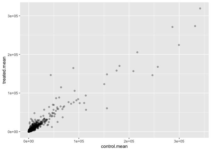
Make a ggplot of average counts of control versus treated
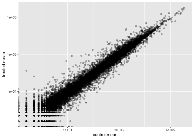
ggplot(meancounts) +
  aes(control.mean, treated.mean) +
  geom_point(alpha = 0.3) +
  scale_x_log10() +
  scale_y_log10()
Warning in scale_x_log10(): log-10 transformation introduced infinite values.

Warning in scale_y_log10(): log-10 transformation introduced infinite values.
Log2 units and fold change
If we consider treated/control counts we will get a number that tells us the change (fold change) is the log of this fraction meaning for instange log(1/1) = 0 therefore no hange while the fraction itself may equal 1. A doublign will lead to +1 log(2) = 1, halving will be -1.
idea - take existing mean counts data frame and make an additional fold change column
log2(10/20)
[1] -1
Add a new column
log2fcfor log2 fold change of treated/control to ourmeancountsobject
meancounts$log2fc <- log2(meancounts$treated.mean/meancounts$control.mean)

head(meancounts)
                control.mean treated.mean      log2fc
ENSG00000000003       900.75       658.00 -0.45303916
ENSG00000000005         0.00         0.00         NaN
ENSG00000000419       520.50       546.00  0.06900279
ENSG00000000457       339.75       316.50 -0.10226805
ENSG00000000460        97.25        78.75 -0.30441833
ENSG00000000938         0.75         0.00        -Inf
zero.vals <- which(meancounts[,1:2]==0, arr.ind=TRUE)

to.rm <- unique(zero.vals[,1])
mycounts <- meancounts[-to.rm,]
head(mycounts)
                control.mean treated.mean      log2fc
ENSG00000000003       900.75       658.00 -0.45303916
ENSG00000000419       520.50       546.00  0.06900279
ENSG00000000457       339.75       316.50 -0.10226805
ENSG00000000460        97.25        78.75 -0.30441833
ENSG00000000971      5219.00      6687.50  0.35769358
ENSG00000001036      2327.00      1785.75 -0.38194109
Q7. What is the purpose of the arr.ind argument in the which() function call above? Why would we then take the first column of the output and need to call the unique() function?
The arr.ind=TRUE helps find indices aka rows and columns where it is TRUE, or for us - having 0 counts. Calling unique() will ensure we don’t count any row twice if it has zero entries in both samples.
Now we can use some fold thresholds to just check for up and downregulation
up.ind <- mycounts$log2fc > 2
down.ind <- mycounts$log2fc < (-2)
Q8
sum(up.ind)
[1] 250
Q9
sum(down.ind)
[1] 367
Q10
We cannot fully tell as the results have not been tested for their significance yet!
Setting up DESeq2
Let’s do this the right way. DESeq2 is an R package specifically for analyzing count-based NGS data like RNA-seq. It is available from Bioconductor. Bioconductor is a project to provide tools for analyzing high-throughput genomic data including RNA-seq, ChIP-seq and arrays. You can explore Bioconductor packages here.
Bioconductor packages usually have great documentation in the form of vignettes. For a great example, take a look at the DESeq2 vignette for analyzing count data. This 40+ page manual is packed full of examples on using DESeq2, importing data, fitting models, creating visualizations, references, etc.
Just like R packages from CRAN, you only need to install Bioconductor packages once (instructions here), then load them every time you start a new R session.
# Load up DESeq2

library(DESeq2)
Loading required package: S4Vectors

Loading required package: stats4

Loading required package: BiocGenerics

Loading required package: generics


Attaching package: 'generics'

The following objects are masked from 'package:base':

    as.difftime, as.factor, as.ordered, intersect, is.element, setdiff,
    setequal, union


Attaching package: 'BiocGenerics'

The following objects are masked from 'package:stats':

    IQR, mad, sd, var, xtabs

The following objects are masked from 'package:base':

    anyDuplicated, aperm, append, as.data.frame, basename, cbind,
    colnames, dirname, do.call, duplicated, eval, evalq, Filter, Find,
    get, grep, grepl, is.unsorted, lapply, Map, mapply, match, mget,
    order, paste, pmax, pmax.int, pmin, pmin.int, Position, rank,
    rbind, Reduce, rownames, sapply, saveRDS, table, tapply, unique,
    unsplit, which.max, which.min


Attaching package: 'S4Vectors'

The following object is masked from 'package:utils':

    findMatches

The following objects are masked from 'package:base':

    expand.grid, I, unname

Loading required package: IRanges

Loading required package: GenomicRanges

Loading required package: Seqinfo

Loading required package: SummarizedExperiment

Loading required package: MatrixGenerics

Loading required package: matrixStats


Attaching package: 'MatrixGenerics'

The following objects are masked from 'package:matrixStats':

    colAlls, colAnyNAs, colAnys, colAvgsPerRowSet, colCollapse,
    colCounts, colCummaxs, colCummins, colCumprods, colCumsums,
    colDiffs, colIQRDiffs, colIQRs, colLogSumExps, colMadDiffs,
    colMads, colMaxs, colMeans2, colMedians, colMins, colOrderStats,
    colProds, colQuantiles, colRanges, colRanks, colSdDiffs, colSds,
    colSums2, colTabulates, colVarDiffs, colVars, colWeightedMads,
    colWeightedMeans, colWeightedMedians, colWeightedSds,
    colWeightedVars, rowAlls, rowAnyNAs, rowAnys, rowAvgsPerColSet,
    rowCollapse, rowCounts, rowCummaxs, rowCummins, rowCumprods,
    rowCumsums, rowDiffs, rowIQRDiffs, rowIQRs, rowLogSumExps,
    rowMadDiffs, rowMads, rowMaxs, rowMeans2, rowMedians, rowMins,
    rowOrderStats, rowProds, rowQuantiles, rowRanges, rowRanks,
    rowSdDiffs, rowSds, rowSums2, rowTabulates, rowVarDiffs, rowVars,
    rowWeightedMads, rowWeightedMeans, rowWeightedMedians,
    rowWeightedSds, rowWeightedVars

Loading required package: Biobase

Welcome to Bioconductor

    Vignettes contain introductory material; view with
    'browseVignettes()'. To cite Bioconductor, see
    'citation("Biobase")', and for packages 'citation("pkgname")'.


Attaching package: 'Biobase'

The following object is masked from 'package:MatrixGenerics':

    rowMedians

The following objects are masked from 'package:matrixStats':

    anyMissing, rowMedians
dds <- DESeqDataSetFromMatrix(countData=counts,
                              colData=metadata,
                              design=~dex)
converting counts to integer mode

Warning in DESeqDataSet(se, design = design, ignoreRank): some variables in
design formula are characters, converting to factors
dds <- DESeq(dds)
estimating size factors

estimating dispersions

gene-wise dispersion estimates

mean-dispersion relationship

final dispersion estimates

fitting model and testing
res <- results(dds)
res
log2 fold change (MLE): dex treated vs control
Wald test p-value: dex treated vs control
DataFrame with 38694 rows and 6 columns
                 baseMean log2FoldChange     lfcSE      stat    pvalue
                <numeric>      <numeric> <numeric> <numeric> <numeric>
ENSG00000000003  747.1942      -0.350703  0.168242 -2.084514 0.0371134
ENSG00000000005    0.0000             NA        NA        NA        NA
ENSG00000000419  520.1342       0.206107  0.101042  2.039828 0.0413675
ENSG00000000457  322.6648       0.024527  0.145134  0.168996 0.8658000
ENSG00000000460   87.6826      -0.147143  0.256995 -0.572550 0.5669497
...                   ...            ...       ...       ...       ...
ENSG00000283115  0.000000             NA        NA        NA        NA
ENSG00000283116  0.000000             NA        NA        NA        NA
ENSG00000283119  0.000000             NA        NA        NA        NA
ENSG00000283120  0.974916       -0.66825   1.69441 -0.394385  0.693297
ENSG00000283123  0.000000             NA        NA        NA        NA
                     padj
                <numeric>
ENSG00000000003  0.163017
ENSG00000000005        NA
ENSG00000000419  0.175937
ENSG00000000457  0.961682
ENSG00000000460  0.815805
...                   ...
ENSG00000283115        NA
ENSG00000283116        NA
ENSG00000283119        NA
ENSG00000283120        NA
ENSG00000283123        NA
We can get some basic summaries tallies using the summary() function
summary(res, alpha = 0.05)
out of 25258 with nonzero total read count
adjusted p-value < 0.05
LFC > 0 (up)       : 1242, 4.9%
LFC < 0 (down)     : 939, 3.7%
outliers [1]       : 142, 0.56%
low counts [2]     : 9971, 39%
(mean count < 10)
[1] see 'cooksCutoff' argument of ?results
[2] see 'independentFiltering' argument of ?results
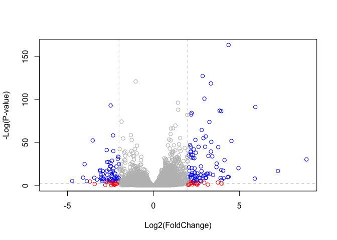
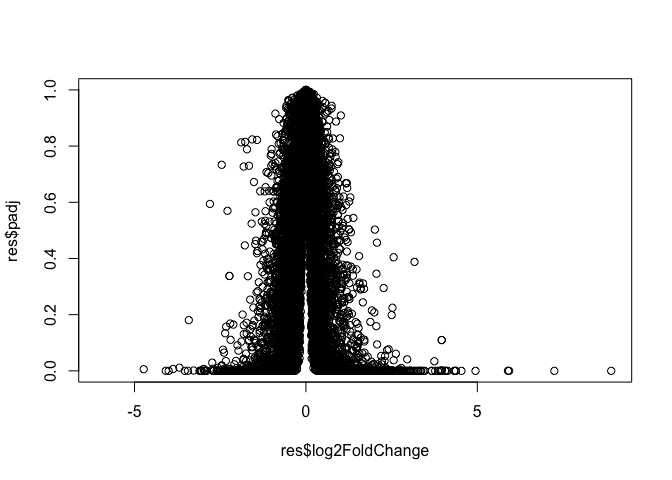
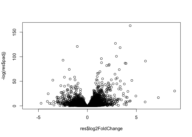
Data Visualization - Volcano plots
plot(res$log2FoldChange, res$padj)
plot(res$log2FoldChange, -log(res$padj))
# Setup our custom point color vector
mycols <- rep("gray", nrow(res))
mycols[ abs(res$log2FoldChange) > 2 ]  <- "red"

inds <- (res$padj < 0.01) & (abs(res$log2FoldChange) > 2 )
mycols[ inds ] <- "blue"

# Volcano plot with custom colors
plot( res$log2FoldChange,  -log(res$padj),
 col=mycols, ylab="-Log(P-value)", xlab="Log2(FoldChange)" )

# Cut-off lines
abline(v=c(-2,2), col="gray", lty=2)
abline(h=-log(0.1), col="gray", lty=2)